Spin Squeezing
PIQS can be used to study spin squeezing and the effect of collective and local processes on a spin squeezing Hamiltonian such as:
which evolves under the dynamics given by:
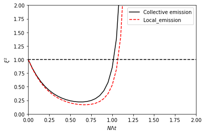
In [1] it has been shown that the collective emmission (\(\gamma_\text{CE}\)) affects the spin squeezing in a system in a different way than the homogeneous local emission (\(\gamma_\text{E}\)). In PIQS, we can study these effects easily by adding these rates to an ensemble constructed as a Dicke object.
from qutip import *
from piqs import *
import matplotlib.pyplot as plt

# general parameters
N = 20
nds = num_dicke_states(N)
[jx, jy, jz] = jspin(N)
jp, jm = jspin(N, "+"), jspin(N, "-")
jpjm = jp*jm

lam = 1
# spin hamiltonian
h = -1j*lam*(jp**2-jm**2)

gamma = 0.2

# Ensemble with collective emission only
ensemble_ce = Dicke(N=N, hamiltonian=h, collective_emission=gamma)

# Ensemble with local emission only
ensemble_le = Dicke(N=N, hamiltonian=h, emission=gamma)

# Build the Liouvillians for both ensembles
liouv_collective = ensemble_ce.liouvillian()
liouv_local = ensemble_le.liouvillian()
Once we have defined our ensembles and constructed their Liouvillians, we can plot the time evolution of the spin squeezing parameter given by \(\xi^2= \frac{N \langle\Delta J_y^2\rangle}{\langle J_z\rangle^2}\) starting from any initial state.
# set initial state for spins (Dicke basis)
rho0 = dicke(N, 10, 10)
t = np.linspace(0, 2.5, 1000)

result_collective = mesolve(liouv_collective, excited(N), t, [],
                 e_ops = [jz, jy, jy**2,jz**2, jx])
result_local = mesolve(liouv_local, excited(N), t, [],
                 e_ops = [jz, jy, jy**2,jz**2, jx])

# Get the expectation values
jzt_c, jyt_c, jy2t_c, jz2t_c, jxt_c = result_collective.expect
jzt_l, jyt_l, jy2t_l, jz2t_l, jxt_l = result_local.expect

del_jy_c = jy2t_c - jyt_c**2
del_jy_l = jy2t_l - jyt_l**2

xi2_c = N * del_jy_c/(jzt_c**2 + jxt_c**2)
xi2_l = N * del_jy_l/(jzt_l**2 + jxt_l**2)

# Generate the plots
plt.plot(t*N*lam, xi2_c, 'k-', label="Collective emission")
plt.plot(t*N*lam, xi2_l, 'r--', label="Local_emission")
plt.plot(t*N*lam, 1+0*t, '--k')
plt.ylabel(r'$\xi^2$')
plt.xlabel(r'$ N \Lambda t$')
plt.legend()

plt.xlim([0, 2])
plt.ylim([0, 2])
plt.show()
References:
- 1
Chase and J. Geremia, Collective processes of an ensemble of spin-1 particles, Phys. Rev. A 78, 052101 2 (2008).