Superradiant Light Emission

We consider a system of \(N\) two-level systems (TLSs) with identical frequency \(\omega_{0}\), which can emit collectively at a rate \(\gamma_\text{CE}\), and suffer from dephasing and local losses at rates \(\gamma_\text{D}\) and \(\gamma_\text{E}\), respectively. The dynamics can be written as

\[\dot{\rho} =-i\lbrack \omega_{0}J_z,\rho \rbrack +\frac{\gamma_\text {CE}}{2}\mathcal{L}_{J_{-}}[\rho] +\sum_{n=1}^{N}\frac{\gamma_\text{D}}{2}\mathcal{L}_{J_{z,n}}[\rho] +\frac{\gamma_\text{E}}{2}\mathcal{L}_{J_{-,n}}[\rho].\]

When \(\gamma_\text{E}=\gamma_\text{D}=0\) this dynamics is the classical superradiant master equation. In this limit, a system initially prepared in the fully-excited state undergoes superradiant light emission whose peak intensity scales proportionally to \(N^2\).

from qutip import *
from piqs import *
import matplotlib.pyplot as plt

N = 20
[jx, jy, jz] = jspin(N)
jp = jspin(N, "+")
jm = jp.dag()

# spin hamiltonian
w0 = 1
H = w0 * jz

# dissipation
gCE, gD, gE = 1, 1, 0

# set initial conditions for spins
system = Dicke(N=N, hamiltonian=h, dephasing=gD,
               collective_emission=gCE)

# build the Liouvillian matrix
liouv = system.liouvillian()

Now that the system Liouvillian is defined, we can use QuTiP to solve the dynamics. We use as integration time a multiple of the superradiant delay time, \(t_\text{D}=\log(N)/(N \gamma_\text{CE})\). We specify the operators for which the expectation values should be calculated to mesolve with the keyword argument e_ops. In this case, we are interested in \(J_x, J_+ J_-, J_z^2\).

nt = 1001
td0 = np.log(N)/(N*gCE)
tmax = 10 * td0

t = np.linspace(0, tmax, nt)

# initial state
excited_rho = excited(N)

# alternative states
superradiant_rho = dicke(N, N/2, 0)
subradiant_rho = dicke(N, 0, 0)
css_symmetric = css(N)

a = 1/np.sqrt(2)
css_antisymmetric = css(N, a, -a)
ghz_rho = ghz(N)
rho0 = excited_rho
result = mesolve(liouv, rho0, t, [], e_ops = [jz, jp*jm, jz**2],
                 options = Options(store_states=True))
rhot = result.states

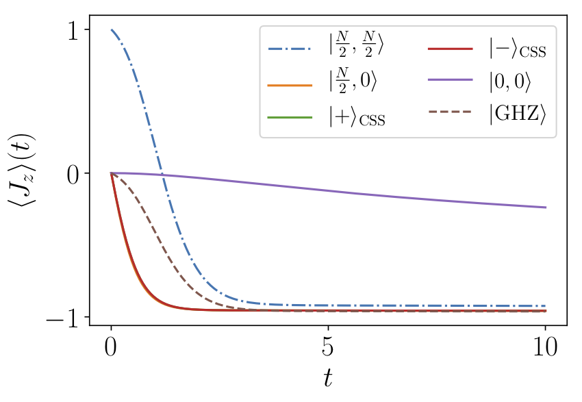
We can then plot the results of the time evolution of the expectation values of the collective spin operators for different initial states.

jz_t = result.expect[0]
jpjm_t = result.expect[1]
jz2_t = result.expect[2]

jmax = (0.5 * N)
fig1 = plt.figure()
plt.plot(t/td0, jz_t/jmax)
plt.show()
plt.close()

References:

1

Dicke, R. H. “Coherence in Spontaneous Radiation Processes”. Phys. Rev. 93, 91 (1954) doi/10.1103/PhysRev.93.99.

2

Bonifacio, R. and Schwendimann, P. and Haake, Fritz. “Quantum Statistical Theory of Superradiance. I.” Phys. Rev. A 4, 302 (1971) doi:10.1103/PhysRevA.4.302